CONTENTS
Graphs: sine, cosine and tangent
OTHER MATERIAL
Wavelength, Frequency and Amplitude
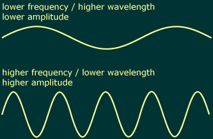
Any wave-like change, such as simple harmonic motion, can be described by two basic characteristics: wavelength and amplitude. Wavelength refers to the speed of the oscillation; amplitude refers to the magnitude of the change.
Specifically, the wavelength of any periodic phenomenon is the distance between successive peaks in the wave. The amplitude is the height of a peak over the wave's baseline (or half the height from peak to trough).

A wave's frequencyis another way to describe its speed, and is equal to the inverse of its wavelength (frequency=1/wavelength). Instead of measuring the interval between successive peaks, frequency measures the number of peaks over a given interval (typically one second).
We can increase the frequency of the trigonometric functions in Javascript by multiplying the values fed to them by some factor. This will make those values change more quickly, thereby increasing the results' frequency. For instance, the wave resulting from Math.sin(time*6) has 6 times the frequency as that from Math.sin(time), because the input values change six times as quickly.
We can increase the amplitude of the wave by multiplying the trigonometric functions' results by some factor. For instance, the wave resulting from 5*Math.sin(time) will have five times the amplitude as that from Math.sine(time)—the former will range from -5 to +5 whereas the latter ranges from -1 to +1.
amplitude*Math.sin(angle*frequency)
Neither amplitude nor frequency has to remain constant throughout the wave's duration. You could, for instance, use a slider value for either factor, and modulate the amplitude or frequency (or both) over the course of the wave. The following diagram illustrates the difference between modulating the frequency and the amplitude of a wave:
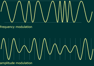
This, by the way, is the basic difference between AM and FM radio: amplitude modulation vs frequency modulation.
Example: Decaying Spring
![]() In
the previous section we used simple harmonic motion to create a spring-like
animation. While the results were acceptable, they failed to decay the
way a real-world spring would. We can now revisit this animation with
an understanding of amplitude and frequency to create a more realistic
effect.
In
the previous section we used simple harmonic motion to create a spring-like
animation. While the results were acceptable, they failed to decay the
way a real-world spring would. We can now revisit this animation with
an understanding of amplitude and frequency to create a more realistic
effect.
The original expression, and resulting animation:
x=Math.sin(time*3)*60;
rest=position;
add(rest, [x,0]);
Our goal is for the spring's motion to slowly decay, until the spring comes to a complete rest. This means we'll need gradually to reduce the amplitude to zero over the course of the animation. In the original expression, we hard-coded the frequency and amplitude (with 3 and 60, respectively), so they remained unchanged throughout the animation. To prepare for our new animation, we'll replace these terms with variables:
frequency=3;
amplitude=60;
x=Math.sin(time*frequency)*amplitude;
rest=position;
add(rest, [x,0]);
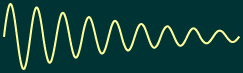
Now, we could try reducing the frequency over the course of the animation, but the results would be unrealistic. The spring would slow down, but still move just as far on each oscillation as before—as though it were moving through molasses. So we'll stick with decreasing the amplitude. A graph of the resulting wave would look like:
So how can we define the variable 'amplitude' so that its value will decrease over time? One way would be to write a simple equation using time as a component, such as "amplitude=60/time." But this would decrease too quickly for our needs, and would generate an error at time=0, because you cannot divide by zero. We'll get better results, with less work, by using the linear() interpolation function:
amplitude=linear(time, 0, out_point-1, 120, 0);
As time goes from zero to one second before the layer's end point, amplitude will decrease from 120 to zero. We're starting with a higher amplitude than before in order to convey a greater feeling of energy. We'll also use a higher (constant) frequency, for the same purpose.
frequency=10;
amplitude=linear(time, 0, out_point-1, 120, 0);
rest=position;
x=Math.sin(time*frequency)*amplitude;
add(rest, [x,0]);
The resulting animation is considerably more realistic than our earlier attempt:
Unfortunately, these results are still not completely realistic—for that, we'd need to accurately calculate the energy stored in the spring at each point and pass this information from frame to frame. Because expressions are 'stateless', with no knowledge of previous or future frames, simulations like this are difficult to achieve. Motion Math, by contrast, is well-suited for tasks like this, and even includes two sample 'spring' scripts ("spring.mm" and "dbspring.mm", in your After Effects application folder). Still, this expression can be very useful in situations where absolute fidelity to the real world isn't necessary.
Click here to download this project. (Windows users click here.)